REMAG
Project 14 · October 2026
REMAG is a GPU-first derivative of SIESTA for magnetic materials. REMAG keeps the electronic state on the GPU, reuses information between self-consistent-field iterations, and reorganizes the most time consuming operations. REMAG is purpose built to be highly performant for fully relativistic, noncollinear calculations with spin–orbit coupling enabled.
The latest REMAG benchmark measures a 14.04× end-to-end speedup for 54-atom iron against a passing upstream ELSI GPU configuration, using strict regression convergence thresholds. Selected native ELPA GPU comparisons range from 17.39× to 110.69×. Comparison runs are limited, and acceleration can vary widely across compounds and configurations. We intend to use this writeup to showcase our optimization strategies, highlight noteable individual comparisons between the native SIESTA GPU paths, and drive further interest in a GPU native future for scientific computing packages. Measurements and scope are below.
REMAG builds on SIESTA 5.4.2. We keep an unmodified, pinned copy as the numerical reference and apply REMAG’s integration patch to a separate source tree. SIESTA supplies the physical model and the executable specification for this independent experimental derivative.
The electronic loop
A density-functional calculation repeats a loop as we know from previous background information that you can read more about here: SCF trajectories article. The loop stops when its convergence criteria are satisfied, magnetic calculations track the magnitude and direction of magnetization, and with spin–orbit coupling, rotating that direction changes the energy giving rise to small differences that require careful convergence.
SIESTA represents the states in localized atomic orbitals. At each sampled wavevector, or k point, it solves
$$H_k C_k = S_k C_k \varepsilon_k,$$where \(H_k\) is the Hamiltonian, \(S_k\) describes orbital overlap, and \(C_k\) and \(\varepsilon_k\) are the states and their energies. Occupying the states produces a density matrix, and contracting it with orbital values on the grid gives the next charge and spin densities.
Upstream SIESTA already leverages ELPA, either directly or through ELSI. In the configurations we measured, the surrounding grid operations, mixing and SCF control remain on the CPU. REMAG brings those operations and their working state onto the GPU. The first diagram compares these two architectures.
Persistant States
Hamiltonian and density matrices, occupation data, mixer history and solver workspace are allocated before the electronic loop. Successive operations consume those buffers directly. CUDA graphs carry the loop, device-side convergence decisions and conditional Pulay mixing. This persistant state removes repeated host orchestration and scalar readbacks along with the larger array transfers.
Reusing the eigensystem
Figures 2–8 isolate REMAG’s kernel and data-layout optimizations. Much of the time spent developing REMAG was autonomous hill climbing with GPT-6 Astra. Our initial implementation was verified against the upstream GPU path, and then Astra was tasked with making iterative improvements to kernels and data structures. The gray panels detail early REMAG implementations, and the pink shows its current replacement.
Independent k-point/spin problems can share a GPU without sharing their working buffers. Each workspace owns its matrices, scratch and results with the pool capped by the available jobs. Eight workspaces added about 94 MiB in the FePt16 comparison.
Major disclaimer here: The timing strips beside these diagrams are separate, matched experiments against the preceding REMAG implementation, each with three fresh paired runs. Builds and A100 variants differ between experiments. These end-to-end gains cannot be multiplied into an upstream-GPU speedup. Individual timings and SCF iteration counts remain in the downloadable data. Floating-point summation order can change those counts, so the timings measure time to equivalent converged solutions.
Successive Hamiltonians tend to be related, so we chose to retain an eigenbasis for each physical k-point/spin job, reorthogonalize it with Cholesky QR, and transform the current Hamiltonian into that basis before continuing the block-Jacobi solve. The saved basis belongs to the job, even when another job reuses its workspace.
Inside the solver, many local problems have only 32 states. A dedicated kernel keeps each real or complex Hermitian matrix and its eigenvectors in one thread block’s shared memory through the Jacobi rotations. Arithmetic here remains FP64.
Density Layout
Several periodic images can refer to the same pair of unit-cell orbitals. Their expensive sum over occupied states is shared where only the phase depends on the image. A unique-pair list and an image-to-pair map let us separate these operations.
The FePt16 maps and scratch cost about 1.04 MB of setup staging and 2.65 MB of cycle memory. Density and energy-density contributions remain sparse, with energy-density retained for forces. The noncollinear symmetrization still follows the periodic phase, and the full SOC spin-component layout is preserved.
Neighboring grid points offer another reuse opportunity. The eight-point cluster kernel shares orbital-pair lookups and density-matrix reads, while keeping each point’s accumulator in registers. Potential assembly similarly shares basis-product work across spin channels with sparse charge reductions distributing a row across a block of threads.
We also changed where arrays originate. Compact neighbor and projector metadata replaces expanded nonlocal query lists in the upload where the GPU then expands them. Initial orbital values and atomic reference fields are generated on the GPU and consumed there. Supported force and population calculations use the retained electronic state, with explicit exports for requested files.
Larger spinor matrices
The 128-atom FePt case has 2,304 spinor states, making for substantial matrix rotation work. REMAG reduces their cost by keeping a tile intermediate in shared memory, using Hermitian symmetry to compute one off-diagonal partner, and grouping complex products into the A100’s FP64 matrix instructions. Real and imaginary parts occupy separate shared-memory planes. Operands and accumulators remain double precision, although addition order does change.
With both contenders already using FP64 vector rotation, enabling FP64 matrix rotation reduced median FePt128 z time from 203.275 to 190.832 seconds: 6.1% less wall time, with all three pairs faster. Direct CPU comparisons, requested exports and the x/z anisotropy check all passed. FePt16 showed no gain (11.011 versus 11.025 seconds), so these large-matrix modes remain opt-in. They were disabled in both benchmark campaigns below.
Measurement also ruled out plausible alternatives. A single library batch of independent eigensystems was slower than the workspace pool. Caching an overlap factor and reducing some local solver block sizes also failed to establish useful gains.
Measured performance
Our brief benchmarking campaign declared seven workflows with prior successful convergence. We ran 49 calculations sequentially on one A100-SXM4-80GB. Screening covered native ELPA and applicable ELSI configurations. The completed comparisons below each have three fresh timing repetitions, with contender order alternated and actual upstream GPU execution verified. Again the benchmarking here is not broad, we are showcasing gains that we measured and intentionally avoiding grandiose claims that would require much more thorough benchmarks.
These speedups use unusually strict stopping thresholds: DM 1e-9 and H 1e-8 eV for both contenders, each 100,000 times tighter than SIESTA’s defaults. We adopted them for stringent numerical regression, including saved-density-matrix agreement after earlier looser runs failed that check. They are benchmark settings, not an established requirement for every REMAG calculation. Both paths also use conservative 0.05 Pulay mixing, six history entries and fresh initial densities.
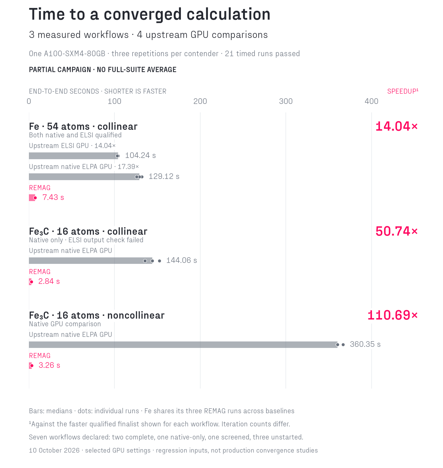
The faster ELSI finalist uses four MPI ranks, one thread per rank and block size 32. The native Fe54 and collinear Fe₃C finalists use one rank, four threads and block 64 with noncollinear Fe₃C using four ranks, one thread and block 32. All use two-stage ELPA. REMAG uses one CPU thread, its workspace pool and eigenbasis reuse. The allocation reserved 16 CPU cores for both contenders. This screens several configurations, and it is not exhaustive upstream tuning.
The 110.69× result includes different convergence trajectories with noncollinear Fe₃C taking 100 upstream iterations versus 71, 65 and 69 for REMAG. Fe54 goes the other way with ELSI taking 79 iterations, while REMAG takes 107, 127 and 114. These are times to equivalent solutions at the highly strict thresholds. Much of the iteration count is a near-converged tail. Noncollinear Fe₃C crosses the default residual limits at step 23 upstream and step 21 in every REMAG repetition. Fe54 reaches them at step 30 with ELSI and steps 46, 51 and 57 with REMAG. Provisioning, builds, diagnostic tracing and evidence retrieval are excluded from both sides.
Pristine CPU SIESTA independently checks energies, densities, eigenvalues, moments, charges, forces, stress and requested matrix exports. All 21 timed calculations pass at the strict thresholds above; the earlier default-threshold estimates are not independently qualified runs. These Fe and Fe₃C comparisons use PBE, an SZP basis, a 100 Ry mesh and 300 K electronic temperature, without SOC. These are numerical regression inputs. Exact inputs, k-point grids, pseudopotential hashes and every timing repetition are downloadable.
Fe₃C’s corrected 16-rank ELSI screens converged but failed the required eigenvalue-output check, leaving its collinear comparison native-only. Fe54’s eight-rank ELSI screen reached the unchanged 200-SCF cap. An earlier passing eight-rank comparison measured 8.37× on A100 PCIe with an earlier REMAG build, and it remains valid under those conditions. Failed screens are retained and excluded from the ratios.
Earlier measurements · separate runs and baseline settings
9 October 2026 · selected native ELPA GPU baselines · median of three repetitions
| Workflow | GPU → REMAG | Speedup |
|---|---|---|
| Fe54 · collinear | 168.48 → 8.02 s | 21.01× |
| Fe16 · noncollinear | 236.38 → 4.88 s | 48.44× |
| Fe₃C · collinear | 154.24 → 3.35 s | 46.04× |
| Fe₂B · full-SOC x/z | 454.37 → 8.32 s | 54.61× |
The four-workflow geometric mean is 40.00×. Fe₂B counts once as an x/z pair. Failed ELSI screens were excluded; this average is specific to the native baselines in that earlier batch.
Standalone comparison with an earlier REMAG build and its recorded native ELPA GPU setting; three repetitions. Excluded from the four-workflow average and the current campaign.
The earlier Fe₂B full-SOC x/z pair passes all six direct directional-energy comparisons:
- E(x)−E(z) is −0.001622 eV at printed precision
- Within the 5 micro-eV tolerance
- Final moment directions pass.
All 30 timed runs in that four-workflow suite pass the direct CPU checks. The standalone FePt16 full-SOC result also has three repetitions, using an earlier REMAG build. No new repeated SOC or anisotropy result comes from the latest campaign. Agreement of large total energies alone would not establish agreement of their small difference.
The larger FePt upstream-GPU result has only one pair and remains provisional as the repeated large-matrix result above measures an incremental REMAG improvement.
What remains
CPU geometry preparation and ionic work remain, along with requested file exports. We do not claim zero total host/device traffic or zero I/O; some library-internal activity has not been measured.
The evidence covers A100 hardware and magnetic regression inputs. Production anisotropy still needs basis, mesh, k-point, smearing and SCF convergence studies. Some benchmark samples such as Fe₄N’s difficult noncollinear settings remain unqualified. The solver’s 4,096-state implementation limit exceeds our largest magnetic qualification of 2,304 states.
Measuring and validating ordinary stopping thresholds, tuning convergence for both contenders, completing the unfinished workflows, and resolving Fe₃C’s ELSI output gap are the next useful measurements. Learned initialization, SCF updates and the GPAW-inspired solver ideas (thank you @jazzloaf) are deferred to a later iteration.
REMAG's experimental source is available on GitHub under GPL-3.0-or-later. The native implementation and development record describe the measured changes. This article's benchmark data includes individual repetitions, baseline configurations, source-record hashes, build identities and known limitations. Results include work completed through 10 October 2026 (Pacific time).