SOC-Enabled SCF Trajectories
Project 14 & SF Compute · September 2026
Our SOC-SCF Trajectories dataset holds 310 self-consistent-field (SCF) histories from spin–orbit-coupled density functional theory calculations performed on select magnetic materials. For each SCF evaluation we store the input charge and spin density, the produced effective potential, and the resulting density.
A special thank you to the SF Compute team. SF Compute provided the compute infrastructure that made this dataset possible. Their nodes supported multiple parallel spin–orbit-coupled Quantum ESPRESSO runs, preserving the charge, spin and potential fields throughout each SCF history. That sustained compute time let us collect both converged solutions and their full trajectory history. To our knowledge, this is the first publicly released dataset of SCF field trajectories for periodic, spin–orbit-coupled DFT.
The dataset is available on Hugging Face at project-14/soc-scf-trajectories under CC BY 4.0.
We intend for this white paper to be a primer as much as a dataset card. If you already work with noncollinear DFT or are familiar with the concepts, feel free to skip to what we built or the use cases. Otherwise the sections below provide some background in the following order: what DFT computes, why the calculation is a loop, collinear and noncollinear spin, spin–orbit coupling, and why magnets need all of it. Every field image and chart is drawn from the released data. The diagrams and the interactive models are labeled as schematic and are intended to be illustrative.
What a DFT calculation computes
A crystal is a periodic lattice of nuclei and their electrons. The electrons in these systems determine almost everything we know about a material. Magnetic properties, bond strength and magnetization direction are all properties that the electrons determine. The Schrödinger equation underpins the behavior of these electrons, but in practice the many-electron wavefunction is unmanageable given it depends on the positions of all the electrons in the system at once. The FeAl₂ cell in Figure 1 has 44 valence electrons, giving rise to a 132-dimensional wavefunction. This is far too expensive to compute.
Hohenberg and Kohn showed that the ground-state electron density \(n(\mathbf r)\), a three-coordinate function, determines the ground-state properties of the system [1]. Kohn and Sham built on this and turned it into a practical method [2] where we can replace the interacting electrons with fictitious non-interacting ones that move in an effective potential, chosen so that they reproduce the same density. In atomic units,
$$\Big[-\tfrac12\nabla^2+v_{\rm eff}[n](\mathbf r)\Big]\psi_i(\mathbf r)=\varepsilon_i\,\psi_i(\mathbf r),\qquad n(\mathbf r)=\sum_i f_i\,|\psi_i(\mathbf r)|^2,$$where the \(\psi_i\) are the Kohn–Sham orbitals and \(f_i\) their occupations. This effective potential has three parts: the attraction of the nuclei, represented by pseudopotentials that replace the core electrons; the classical electrostatic (Hartree) repulsion of the density; and exchange and correlation. The last of these carries the rest of the quantum mechanics (it is not known exactly and must be approximated). Every calculation in this dataset uses the PBE generalized-gradient approximation [3].
Self-consistency
The Kohn–Sham problem is circular (think of a circular reference in Excel, it’s the exact same concept). The potential depends on the density, but the density comes from the orbitals, which depend on the potential. A calculation must therefore start from an initial guess and iterate:
- Build the effective potential from an input density
- Solve the Kohn–Sham equations for orbitals in that potential
- Sum the occupied orbitals into an output density
- Compare the output with the input. If they agree within a tolerance, call it converged and stop. Otherwise, combine them into a new input and repeat.
This is the self-consistent-field (SCF) loop. We’re searching for a fixed point \(n = F(n)\), where \(F\) maps an input density to the output density it produces. The mismatch \(R = F(n) - n\) is the residual. Often times, feeding the output straight back in oscillates or diverges, so solvers take damped steps,
$$n_{k+1}=n_k+\alpha\,\big(F(n_k)-n_k\big),\qquad 0<\alpha\le1,$$and use the history of earlier steps to choose better ones. Pulay’s DIIS [4] and Broyden-type methods [5] are the standard tools, often combined with preconditioners such as Kerker’s, which damps long-wavelength charge sloshing [6]. Woods, Payne and Hasnip review the field [7].
There are two things we want to clarify here. The iteration axis is not time. An SCF history is a sequence of numerical guesses at fixed atomic positions, not electrons moving, and normally only the endpoint survives. Quantum ESPRESSO, like most DFT packages, keeps the latest density for restarts and discards the path entirely.
Collinear and noncollinear spin
Electrons carry spin. Spin is an intrinsic angular momentum with an attached magnetic moment. In most materials spin-up and spin-down electrons pair off and their moments cancel. In iron, cobalt, nickel and many of their compounds they do not. This imbalance is the magnetization.
One way to include spin in DFT calculations is the collinear, spin-polarized scheme of von Barth and Hedin [8]. It picks a single axis and treats spin-up and spin-down electrons as two populations with densities \(n_\uparrow\) and \(n_\downarrow\). The charge density is their sum, \(n = n_\uparrow + n_\downarrow\), and the magnetization density is their difference, \(m = n_\uparrow - n_\downarrow\). Every local moment in the crystal is then parallel or antiparallel to that one axis.
A noncollinear calculation lifts the restriction [9, 10]. Each orbital becomes a two-component spinor, and the density at each point becomes a 2 × 2 matrix:
$$\rho(\mathbf r)=\tfrac12\big[n(\mathbf r)\,\mathbb 1+\mathbf m(\mathbf r)\cdot\boldsymbol\sigma\big],\qquad \psi_i=\begin{pmatrix}\psi_{i\uparrow}\\ \psi_{i\downarrow}\end{pmatrix},$$where \(\boldsymbol\sigma\) are the Pauli matrices. Now four real numbers per point, \((n, m_x, m_y, m_z)\), describe the electrons. In this configuration the magnetization can point in any direction and change direction from place to place. Plane-wave and all-electron codes implement this routinely [11, 12]. The effective potential takes the same form with a scalar part \(V_0\) plus a spin-dependent part \(\mathbf B\cdot\boldsymbol\sigma\). These describe the four potential channels in the dataset.
Without spin–orbit coupling, spin and space are decoupled. You could rotate every spin in the crystal by the same angle and the energy would not change [13]. In a collinear calculation the choice of axis is therefore arbitrary, and so is the direction of a ferromagnet’s magnetization relative to its crystal. Real magnets do not behave like this. Spin–orbit coupling is what ties the spin to the magnet’s lattice.
Spin–orbit coupling
Spin–orbit coupling is a relativistic effect. An electron moving through the electric field of a nucleus experiences, in its own rest frame, a magnetic field proportional to its orbital angular momentum \(\mathbf L\). Its spin \(\mathbf S\) couples to that field (Figure 4). For an electron in a central potential \(V(r)\) the result is
$$H_{\rm SO}=\xi(r)\,\mathbf L\cdot\mathbf S,\qquad \xi(r)=\frac{1}{2m_e^2c^2}\,\frac1r\frac{dV}{dr}.$$Because \(\xi\) follows the slope of the potential, it is largest close to the nucleus and grows rapidly with nuclear charge. For hydrogen-like ions the splitting scales as \(Z^4/n^3\) [14]. Screening by inner electrons slows this growth for valence electrons in solids. SOC is modest in 3d metals such as iron and several times larger in 4d and 5d elements such as palladium and platinum (Figure 5) [15].
Spin–orbit coupling has two direct consequences that impact this dataset.
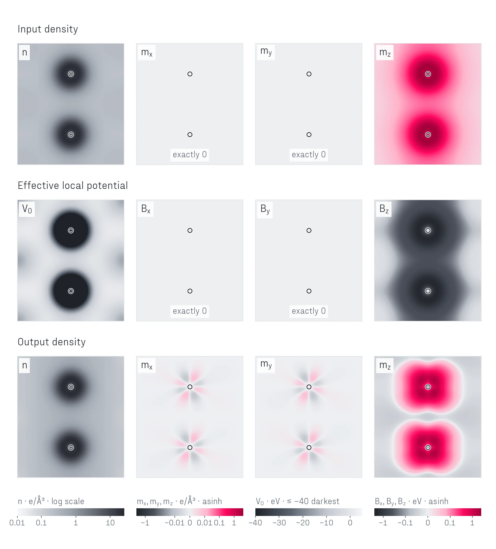
It makes the calculation noncollinear. Take \(\mathbf L\cdot\mathbf S = L_zS_z + \tfrac12(L_+S_- + L_-S_+)\). The second term flips a spin while changing the orbital angular momentum, so it mixes the spin-up and spin-down components of every state. Spin along a fixed axis is therefore no longer conserved, and a calculation with SOC has to work with spinors and a vector magnetization. In Quantum ESPRESSO that means noncollinear spinors plus fully relativistic pseudopotentials that carry the spin–orbit term [16, 17]. Figure 6 shows the effect in our data. The FeAl₂ history starts with its magnetization strictly along \(z\), so the input \(m_x\) and \(m_y\) are exactly zero, as are \(B_x\) and \(B_y\). One solve later the output has transverse spin density around each Fe atom. By contrast, a collinear calculation would set these components to zero by construction.
It ties the magnetization to the crystal. Through \(\mathbf L\), the spin now ‘feels’ the shape of the electronic orbitals, and those orbitals are fixed by the crystal. The energy therefore depends on which way the magnetization points relative to the crystal axes. This is magnetocrystalline anisotropy (MAE). Van Vleck first traced MAE to spin–orbit coupling [18], and Bruno later connected its size to how the orbital moment changes with direction [19].
The impact on magnets
Permanent magnet performance depends on the magnet’s peak magnetic strength, its ability to retain that magnetism at high temperatures, and its ability to resist being demagnetized. This resistance to demagnetization is dependent on something called anisotropy in the magnet, or the energy cost of pointing the magnetization along different crystal axes. An easy axis gives the magnetization two stable directions that are separated by an energy barrier. To evaluate this barrier, a widely used criterion is the magnetic hardness
$$\kappa=\sqrt{\frac{K_1}{\mu_0M_s^2}}>1,$$where \(K_1\) is the anisotropy constant and \(M_s\) the saturation magnetization [20, 21]. Anisotropy is not sufficient on its own, since coercivity also depends heavily on microstructure, lattice defects and operating temperature [22]. This anisotropy is still a required property. Without it you have no permanent magnet.
Interactive · schematic energy model
Model: E(θ) − E(0) = K sin²θ with K > 0 when SOC is on and K = 0 when it is off, in units of K. Real anisotropy energies are microelectronvolts to about a millielectronvolt per atom and are computed, not assumed. Shape (dipolar) anisotropy and higher-order terms are omitted.
The ‘best’ (probably better phrased as most performant and widely used) magnets today, Nd₂Fe₁₄B and SmCo₅, get their anisotropy from the strong spin–orbit coupling of rare-earth 4f electrons [23]. Their supply is concentrated, as has become all too topical in recent years. China mined about 270,000 of an estimated 390,000 tonnes of rare-earth oxide in 2025 [24], and a 2022 U.S. Department of Energy assessment put its share of global rare-earth magnet production at 92% [25]. American startups and other global rare-earth mining and refinement companies are cutting into this market share. Rare-earth-free candidates attempt to combine the magnetization of 3d elements such as iron, cobalt and manganese with anisotropy from crystal structure and from heavier elements with stronger SOC [26, 22]. To properly screen a rare-earth-free permanent magnet candidate, we need to run these SOC-enabled calculations.
Those calculations are expensive, and often tricky to compute. The anisotropy energy is extremely small. Measured values for bcc iron, hcp cobalt and fcc nickel, as compiled by Xie and Blackman, are 1.4, 65 and −2.7 μeV per atom [27]. Even L1₀ FePt, a benchmark hard magnet, reaches only about 1.8 meV per FePt pair [28]. To attempt to compute this anisotropy value directly, compounds need to be ‘converged’ (more on this later) far beyond the energy threshold of what will ultimately be a small difference between two large energies corresponding to different magnetization axes. Early first-principles work on iron, cobalt and nickel showed how demanding this process is [29, 30] (force-theorem methods estimate the difference from band energies at a fixed potential [31, 32]).

Shown above (Figure 7), the total energy drops below the scale of iron’s anisotropy by evaluation 15 before the density has converged. The total energy is stationary at the solution, so its error shrinks faster than the density error, and quantities that depend on the density or the magnetization directly converge more slowly.
Our dataset
We ran 310 SCF histories with spin–orbit coupling on candidate magnetic materials, using a GPU-accelerated build of Quantum ESPRESSO instrumented to write out its fields at every evaluation step. The result is SOC-SCF Trajectories [33]. For every evaluation it contains:
- the input density \((n, m_x, m_y, m_z)\) on the calculation’s native real-space grid;
- the effective local potential \((V_0, B_x, B_y, B_z)\) built from it;
- the output density \((n, m_x, m_y, m_z)\) from the spinor Kohn–Sham solve;
- scalar diagnostics: charge and spin residuals, band and smearing energies, Fermi level and the net spin vector, plus the total energy that Quantum ESPRESSO reported for about half of the evaluations.
Each history also carries its crystal structure, the retained Quantum ESPRESSO input, its numerical settings and starting magnetization, an outcome label, a structural family and a frozen train, validation or test split.
To our knowledge, this is the first publicly released dataset of SCF field trajectories for periodic, spin–orbit-coupled DFT. At every SCF evaluation it preserves the input and output charge and vector-spin densities together with the effective local potential, on the native real-space grid.
We did search for counterexamples. The closest public data we found are density coefficients sampled along SCF trajectories for closed-shell molecules, released with NeuralSCF [34]; they contain no spin density and no crystals. Public crystalline density databases, such as the Materials Project charge-density collection, store converged densities that are at most collinear [35]. Public spin–orbit datasets for machine learning, such as Materials-HAM-SOC, store Hamiltonians rather than field trajectories [36]. Potential-to-density training pairs for crystals, including unconverged steps, have been generated with Quantum ESPRESSO to learn the Kohn–Sham map [37]; that work does not describe spin channels, and we did not find a public release of its fields. The claim therefore depends on the combination: iteration-resolved density data by itself is not new.
| Part of a record | How to read it |
|---|---|
| Density \(n\), \(m_x\), \(m_y\), \(m_z\) | Charge and spin density in electrons/ų. Spin density uses electron-density units; integrating \(\mathbf m\) over the cell gives the spin moment in Bohr magnetons. |
| Potential \(V_0\), \(B_x\), \(B_y\), \(B_z\) | The local part of the effective potential, in eV. The B channels are energy coefficients, not a magnetic field in tesla. |
| What the potential omits | The nonlocal pseudopotential terms, which carry the spin–orbit coupling itself. The four local channels are not the whole Hamiltonian. |
| Density type | Pseudo-valence density from norm-conserving pseudopotentials, not an all-electron density. |
| Grid and frame | Arrays of shape (4, nz, ny, nx), C order with x fastest, on the native grid of each cell. Spin components use a Cartesian frame. |
The spin–orbit signal in the densities is small but it is present. In the final FeAl₂ evaluation the transverse spin density peaks at about 1% of the peak \(m_z\), and it sums to zero over the cell. Also, with LDA- and GGA-type functionals the exchange–correlation field is locally parallel or antiparallel to the magnetization [38, 39]. In that same evaluation, \(\mathbf B\) is collinear with \(\mathbf m\) at every grid point where \(|\mathbf m|\) exceeds 1% of its peak, and antiparallel at 99.1% of them. Opposite local contributions can also cancel. The FeAl₂ cell’s net spin moment is 4.04 μB, while \(\int|\mathbf m|\,d\mathbf r\) is 4.81, because regions of negative \(m_z\) hold −0.38 electrons’ worth of spin.
Interactive · measured fields from the dataset
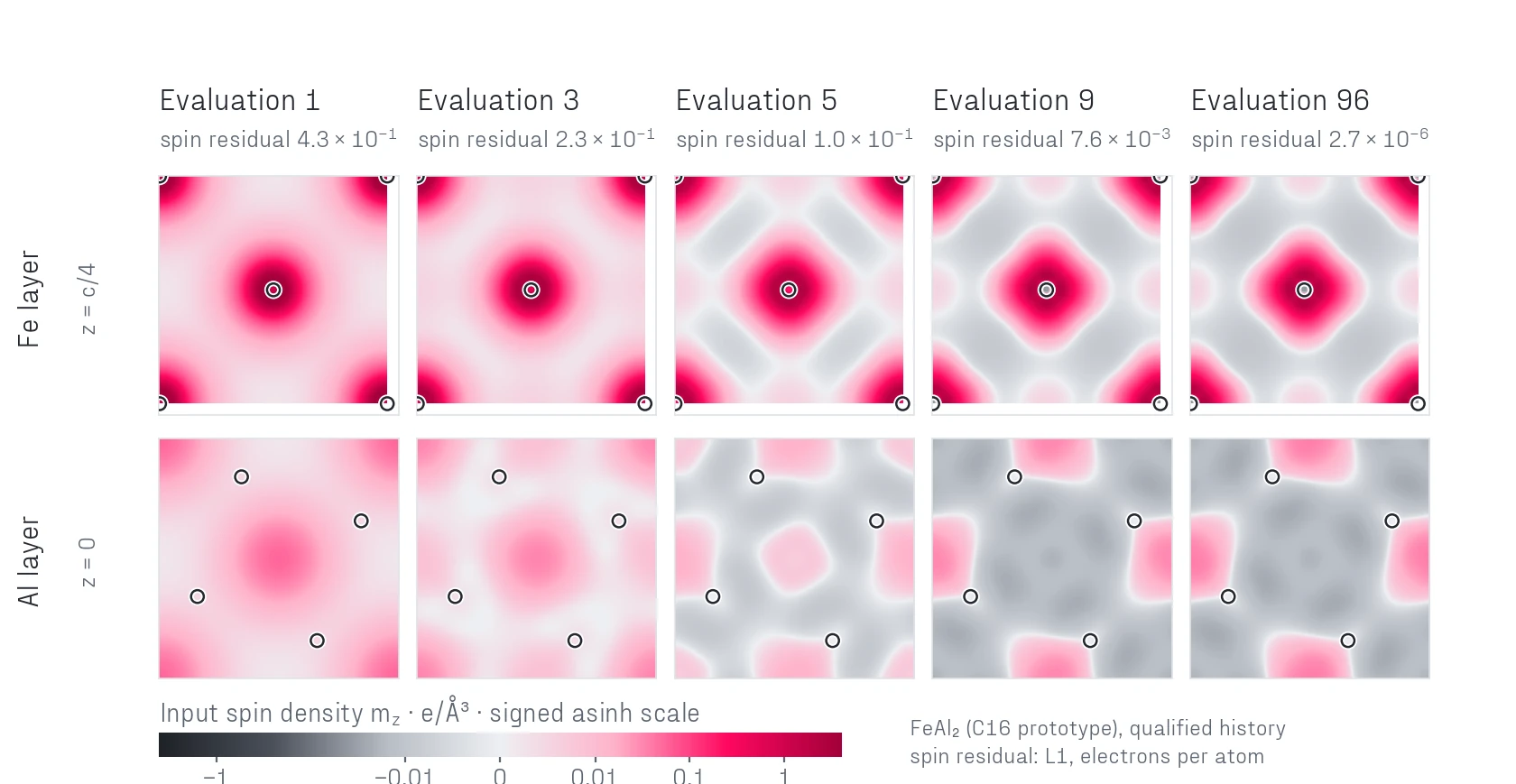
FeAl₂, trajectory proto014-feal2-reference130-002. Images are two slices through the same record: a layer containing Fe atoms and a layer containing Al atoms.
Each image is one conventional-cell slice (6.04 Å square), resampled from the record's 72 × 72 × 72 grid. Open circles mark atoms in the slice. The residual chart covers all 96 evaluations; images are provided for evaluations 1–9 and the final evaluation, 96. Color scales are fixed across evaluations so magnitudes can be compared.
Things to look for in the explorer. With Input spin selected, step from evaluation 1 to 9 and watch negative spin (gray) appear in the Al layer; it was not in the starting guess. Spin residual and charge residual show where input and output disagree. The residuals shrink by five to six orders of magnitude, and the part that remains concentrates around the Fe atoms. Potential V₀ barely changes, because it is dominated by the fixed pseudopotential wells around each atom.
What the histories show
Spin settles more slowly than charge. The final spin residual exceeds the final charge residual in 308 of the 310 histories. That fits a known asymmetry in magnetic SCF calculations. Preconditioners such as Kerker’s act on long-wavelength charge fluctuations, but spin density interacts only through the exchange–correlation kernel and is not preconditioned in that way [7].
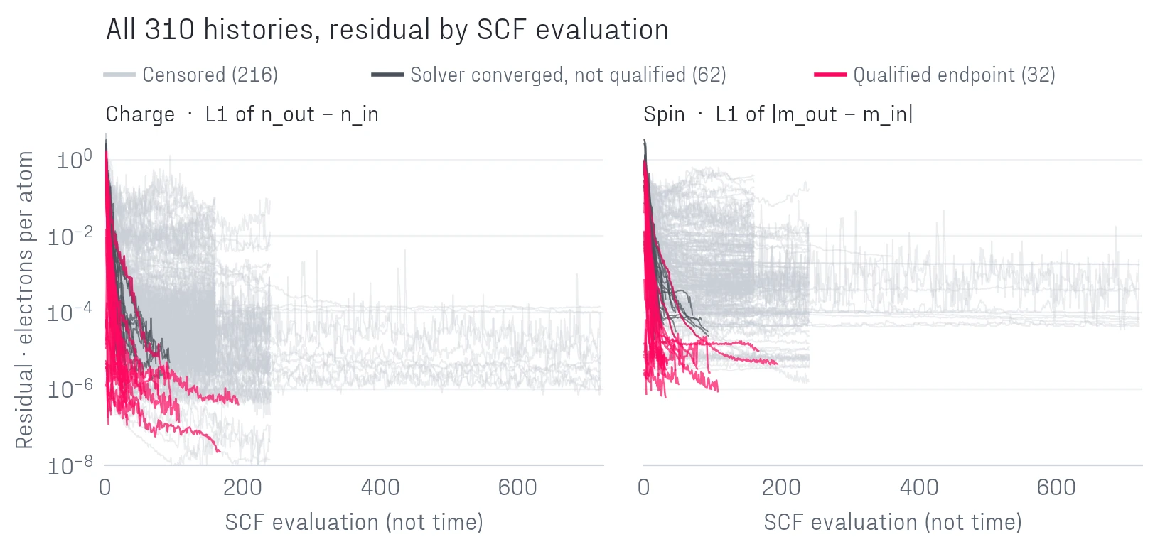
Progress is not monotone. In 282 out of 310 histories, the residual rises at least once between adjacent evaluations, with some histories settling in a few dozen steps. Others, like the FeAl₂ run in Figure 7, stall on long plateaus which sit near 10⁻⁵ electrons per atom for about 70 evaluations before a final drop.
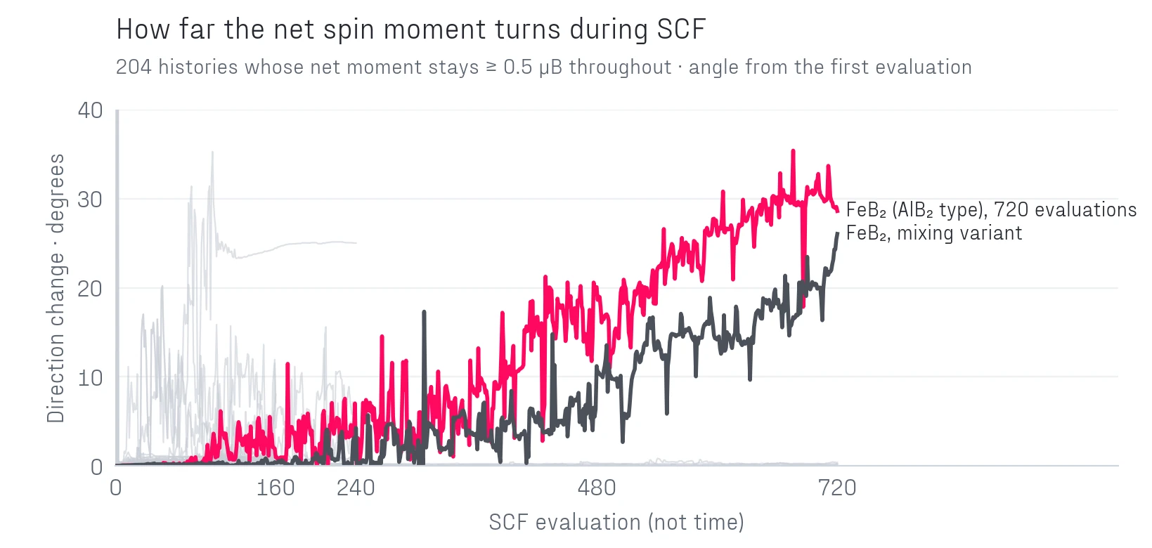
The moment’s direction is a slow coordinate. Anisotropy energies are small. Very little energy favors one magnetization direction over another, and the solver has very little to push against. In 197 of the 204 histories whose net moment stays above 0.5 μB, the moment ends within 2° of the starting direction. Two FeB₂ histories turn by 26–29° over 720 evaluations without converging (Figure 9). The trajectory here is informative as the endpoint alone cannot tell you whether a run kept its starting direction.
Coverage and outcomes
Histories have one of three outcomes. A qualified endpoint converged and its final state passed independent electronic checks. Solver converged means Quantum ESPRESSO reported convergence but the endpoint was not independently qualified. Censored histories stopped first, almost always at the iteration limit set in their input. Censoring here does not claim that a system cannot converge.
It’s worth knowing the limits of the coverage before working with the dataset:
- A qualified endpoint is an electronic solution at the recorded geometry and settings. It is not a proven magnetic ground state, a relaxed structure or a material-property label.
- 306 of the 310 histories use 8 k-points, a coarse 2×2×2 mesh. That is enough to study SCF behavior but far too coarse for converged anisotropy energies.
- 14 of the 22 structural families have no qualified endpoint. All 32 qualified endpoints started from a single magnetic species (31) or from parallel moments (1); none started from opposed or nonparallel moments.
- Evaluations within a history are strongly correlated. The 47,198 distinct maps are not 47,198 independent materials.
Coverage across the 22 structural families


Use cases
Most electronic-structure datasets record final outputs such as a converged density, an energy, or a Hamiltonian. This dataset specifically records the map the calculation iterates on, sampled away from its answer, for magnetic systems with spin–orbit coupling, and it preserves the runs that failed. Here we pose two potential questions that could be explored using this data.
Recovering response operators from trajectories
Can you recover useful response operators from trajectories alone, and can a model learn them across structures?
If we nudge the potential that a crystal’s electrons experience, their density shifts, and it’s this static response that underlies screening, phonons and magnetic excitations. This is normally computed with dedicated linear-response methods such as density-functional perturbation theory [40], and for magnets, the spin component of the same response is where spin fluctuations and exchange interactions originate [41].
This same response governs the SCF loop. Near the solution, a damped step multiplies each error mode by \(1-\alpha\lambda\), where \(\lambda\) is an eigenvalue of the dielectric operator \(1-\chi_0K\) [42, 7]. Here \(\chi_0\) is the Kohn–Sham response (potential to density) and \(K\) the Hartree and exchange–correlation kernel (density to potential). Charge sloshing makes some \(\lambda\) large, which forces small steps. Soft magnetic modes make others small, so they barely move. Without spin–orbit coupling enabled, turning the whole magnetization costs nothing and its \(\lambda\) is exactly zero; spin–orbit coupling lifts it only as far as the tiny anisotropy energy allows. Good preconditioners are, at heart, approximations to \(\chi_0\) [43].
Because the dataset stores the potential between the two densities, each history samples both halves of that product:
$$\delta V\approx K\,\delta n_{\rm in},\qquad \delta n_{\rm out}\approx\chi_0\,\delta V,\qquad \frac{\partial F}{\partial n}=\chi_0K,$$where \(\delta\) is the difference between two evaluations of the same history. The nonlocal pseudopotential terms, including spin–orbit coupling, do not change during a run, so the stored local potential carries every change in the Hamiltonian from one evaluation to the next. The densities have four components, so \(\chi_0\) couples charge and spin, and spin–orbit coupling couples the spin directions to one another.
An experiment could proceed in two steps:
- Within one history, fit \(K\) and \(\chi_0\) on the subspace the solver explored, which Broyden-type mixers do implicitly [5], and use them to predict held-out evaluations. Then ask which modes are recovered, and whether the soft ones are spin modes or rotations of the moment.
- Across structures, train a machine learning model conditioned on the crystal to predict \(\chi_0\) acting on a potential change, and test it on the frozen test families. Neural operators have been trained on the potential-to-density map for systems without spin [37]; this dataset adds the spin channels and spin–orbit coupling.
Limits to consider:
- Each history probes only the directions its solver explored, so a recovered operator is low-rank and biased toward the modes that mattered in that run.
- The orbital solve has its own tolerance, which sets a noise floor on small differences.
- Successive evaluations are strongly correlated, so the effective sample is closer to 163 geometries than to 49,007 maps.
Learned mixing for stuck magnetic runs
Can a learned mixer or preconditioner, trained on trajectories, rescue runs that standard Broyden mixing leaves stuck, on structural families it never saw?
Standard mixing handles charge well. Kerker-type preconditioners tame long-wavelength sloshing [6], and adaptive damping makes the step length robust [44]. Spin is harder, because it is not preconditioned the same way [7]. The final spin residual exceeds the charge residual in 308 of 310 histories. Of the 145 histories that keep a net moment of at least 0.5 μB for 40 or more evaluations, 14 were still turning, by more than 0.5° over the second half of the run. None of those 14 qualified, and their median final spin residual was about nine times higher than the others’. Figure 13 shows one of them. After 60 evaluations the FeB₂ spin residual stops improving, fluctuating between about 3 × 10⁻⁵ and 3 × 10⁻² at a median of 28 times the charge residual, while the moment turns by 29°.

That points to a specific design where one could imagine a preconditioner that treats charge, longitudinal spin and the soft transverse modes differently. This preconditioner’s parameters could be learned from the trajectories that converged and from stalled trajectories like the 216 histories we have in our dataset.
This question cannot be answered offline. The dataset does not store orbitals and the mixer’s internal state, so a new mixer cannot be replayed on our recorded data. An honest test would run Quantum ESPRESSO live:
- Train only on the training families.
- Keeping every other setting fixed, take censored histories from the test families and restart each from its retained input with the learned mixer. The pseudopotential files are not redistributed, so this step needs the same QE pseudopotentials.
- Compare against Broyden mixing and a strong non-learned baseline such as adaptive damping [44]. Report the fraction of runs that reach a qualified endpoint, the evaluations needed, and whether the endpoint matches with the same energy, moment and moment direction.
One-step accuracy should not be the goal here. A mixer that predicts the next density well can still be unstable inside the loop. Here we’re looking for an increase in the number of qualified runs per GPU-hour.
Using the dataset
The metadata is small enough to download whole. The fields are large enough that they are likely not small enough to download whole. Start from the metadata, choose the histories you want, then fetch only the shards they need.
| Path | Contents |
|---|---|
metadata/trajectories.jsonl | One row per history: cell, grid, settings, starting magnetization, outcome, family and split. |
metadata/occurrences.jsonl.gz | One row per evaluation, with its residual and the SHA-256 of its three fields. |
metadata/scalar-histories.jsonl.gz | Per-evaluation diagnostics: component residuals, energies, Fermi level, net spin vector. |
metadata/routes/*.json | Per-history index of field sizes, hashes, encodings and grids. |
metadata/inputs/*.in | The retained Quantum ESPRESSO inputs. |
metadata/fields.jsonl.gz | Lookup from each field to its raw shard. |
raw/shard-*.tar.zst | Lossless float64 fields, about 1 GiB per shard. |
The first shard holds the final FeAl₂ evaluation used throughout this page. The repository’s reader downloads only that shard, checks every hash and verifies the 44 electrons in each density:
pip install numpy zstandard huggingface_hub
hf download project-14/soc-scf-trajectories read_example.py --repo-type dataset --local-dir soc-example
python soc-example/read_example.py
Some practical guidance:
- Keep the splits. Train, validation and test are fixed by structural family (198, 43 and 69 histories). Randomly splitting evaluations leaks near-duplicates across the split.
- Keep the order. Canonical map identities bind the potential and output density but not the input, so convergence analysis needs the ordered evaluations.
- Good uses include spatial structure of charge and spin residuals, convergence diagnostics and stopping rules, compression and representation of vector fields, learned density-to-density or potential-to-density maps, and mixing or preconditioning research for noncollinear magnets.
- Limits: orbitals and mixer states are not stored, so exact replay of a history is not possible. Independent orbital reconstruction was done for selected final maps, not every intermediate one. A good one-step prediction does not by itself show stable iterative use or a speed-up.
Release status. The release is complete: all metadata and all 1,368 raw shards (1.46 TB) are published, each checked against its SHA-256 after upload, as recorded in RAW_STATUS.json. Data, metadata and the example reader are released under CC BY 4.0; please cite the exact repository revision you use. The license does not cover Quantum ESPRESSO or third-party pseudopotentials, neither of which is redistributed.
@misc{project14_soc_scf_trajectories_2026,
  author = {{Project 14}},
  title  = {SOC-SCF Trajectories},
  year   = {2026},
  url    = {https://huggingface.co/datasets/project-14/soc-scf-trajectories},
  note   = {Cite the exact dataset revision; CC BY 4.0}
}
Collection
Every history was computed with Quantum ESPRESSO’s plane-wave code [45, 46], running on Nvidia H100 GPUs [47] and instrumented to write the three fields at each evaluation. Common settings: PBE exchange and correlation; fully relativistic norm-conserving pseudopotentials; 120 Ry wavefunction and 480 Ry density cutoffs; Marzari–Vanderbilt smearing (0.01 Ry in 291 histories); and symmetry disabled, so magnetization was free to take any direction. Density mixing used Quantum ESPRESSO’s Broyden scheme in 304 histories and its local Thomas–Fermi variant in 6, with a mixing factor of 0.3 in 265 histories. Starting magnetizations, geometries, mixing and smearing were varied on purpose, so read each history’s input rather than assuming a default. GPU time came from SF Compute.
Field images and dataset charts on this page are generated from the public release by docs/editorial/generate_soc_scf_figures.py in this site's repository. Every residual it recomputes from the raw fields matches the published scalar history.
References
- P. Hohenberg, W. Kohn. Inhomogeneous electron gas. Physical Review 136, B864 (1964). doi:10.1103/PhysRev.136.B864
- W. Kohn, L. J. Sham. Self-consistent equations including exchange and correlation effects. Physical Review 140, A1133 (1965). doi:10.1103/PhysRev.140.A1133
- J. P. Perdew, K. Burke, M. Ernzerhof. Generalized gradient approximation made simple. Physical Review Letters 77, 3865 (1996). doi:10.1103/PhysRevLett.77.3865
- P. Pulay. Convergence acceleration of iterative sequences. The case of SCF iteration. Chemical Physics Letters 73, 393 (1980). doi:10.1016/0009-2614(80)80396-4
- D. D. Johnson. Modified Broyden's method for accelerating convergence in self-consistent calculations. Physical Review B 38, 12807 (1988). doi:10.1103/PhysRevB.38.12807
- G. P. Kerker. Efficient iteration scheme for self-consistent pseudopotential calculations. Physical Review B 23, 3082 (1981). doi:10.1103/PhysRevB.23.3082
- N. D. Woods, M. C. Payne, P. J. Hasnip. Computing the self-consistent field in Kohn–Sham density functional theory. Journal of Physics: Condensed Matter 31, 453001 (2019). doi:10.1088/1361-648X/ab31c0
- U. von Barth, L. Hedin. A local exchange-correlation potential for the spin polarized case. I. Journal of Physics C: Solid State Physics 5, 1629 (1972). doi:10.1088/0022-3719/5/13/012
- J. Kübler, K.-H. Höck, J. Sticht, A. R. Williams. Density functional theory of non-collinear magnetism. Journal of Physics F: Metal Physics 18, 469 (1988). doi:10.1088/0305-4608/18/3/018
- L. M. Sandratskii. Noncollinear magnetism in itinerant-electron systems: theory and applications. Advances in Physics 47, 91 (1998). doi:10.1080/000187398243573
- D. Hobbs, G. Kresse, J. Hafner. Fully unconstrained noncollinear magnetism within the projector augmented-wave method. Physical Review B 62, 11556 (2000). doi:10.1103/PhysRevB.62.11556
- Ph. Kurz, F. Förster, L. Nordström, G. Bihlmayer, S. Blügel. Ab initio treatment of noncollinear magnets with the full-potential linearized augmented plane wave method. Physical Review B 69, 024415 (2004). doi:10.1103/PhysRevB.69.024415
- O. Šipr, S. Mankovsky, S. Polesya et al. Illustrative view on the magnetocrystalline anisotropy of adatoms and monolayers. Physical Review B 93, 174409 (2016). doi:10.1103/PhysRevB.93.174409
- H. A. Bethe, E. E. Salpeter. Quantum Mechanics of One- and Two-Electron Atoms. Springer (1957). doi:10.1007/978-3-662-12869-5
- M. Blanco-Rey, J. I. Cerdá, A. Arnau. Validity of perturbative methods to treat the spin–orbit interaction: application to magnetocrystalline anisotropy. New Journal of Physics 21, 073054 (2019). doi:10.1088/1367-2630/ab3060
- G. Theurich, N. A. Hill. Self-consistent treatment of spin-orbit coupling in solids using relativistic fully separable ab initio pseudopotentials. Physical Review B 64, 073106 (2001). doi:10.1103/PhysRevB.64.073106
- A. Dal Corso, A. Mosca Conte. Spin-orbit coupling with ultrasoft pseudopotentials: application to Au and Pt. Physical Review B 71, 115106 (2005). doi:10.1103/PhysRevB.71.115106
- J. H. Van Vleck. On the anisotropy of cubic ferromagnetic crystals. Physical Review 52, 1178 (1937). doi:10.1103/PhysRev.52.1178
- P. Bruno. Tight-binding approach to the orbital magnetic moment and magnetocrystalline anisotropy of transition-metal monolayers. Physical Review B 39, 865 (1989). doi:10.1103/PhysRevB.39.865
- J. M. D. Coey. Hard magnetic materials: a perspective. IEEE Transactions on Magnetics 47, 4671 (2011). doi:10.1109/TMAG.2011.2166975
- R. Skomski, J. M. D. Coey. Magnetic anisotropy — how much is enough for a permanent magnet? Scripta Materialia 112, 3 (2016). doi:10.1016/j.scriptamat.2015.09.021
- R. W. McCallum, L. H. Lewis, R. Skomski et al. Practical aspects of modern and future permanent magnets. Annual Review of Materials Research 44, 451 (2014). doi:10.1146/annurev-matsci-070813-113457
- J. M. D. Coey. Perspective and prospects for rare earth permanent magnets. Engineering 6, 119 (2020). doi:10.1016/j.eng.2018.11.034
- U.S. Geological Survey. Mineral commodity summaries 2026 (rare earths). U.S. Geological Survey (2026). doi:10.3133/mcs2026
- B. J. Smith, M. E. Riddle et al. Rare earth permanent magnets: supply chain deep dive assessment. U.S. Department of Energy (2022). doi:10.2172/1871577
- O. Gutfleisch, M. A. Willard, E. Brück et al. Magnetic materials and devices for the 21st century: stronger, lighter, and more energy efficient. Advanced Materials 23, 821 (2011). doi:10.1002/adma.201002180
- Y. Xie, J. A. Blackman. Magnetocrystalline anisotropy and orbital polarization in ferromagnetic transition metals. Physical Review B 69, 172407 (2004). doi:10.1103/PhysRevB.69.172407
- J. B. Staunton, S. Ostanin, S. S. A. Razee et al. Temperature dependent magnetic anisotropy in metallic magnets from an ab initio electronic structure theory: L1₀-ordered FePt. Physical Review Letters 93, 257204 (2004). doi:10.1103/PhysRevLett.93.257204
- G. H. O. Daalderop, P. J. Kelly, M. F. H. Schuurmans. First-principles calculation of the magnetocrystalline anisotropy energy of iron, cobalt, and nickel. Physical Review B 41, 11919 (1990). doi:10.1103/PhysRevB.41.11919
- S. V. Halilov, A. Y. Perlov, P. M. Oppeneer et al. Magnetocrystalline anisotropy energy in cubic Fe, Co, and Ni: applicability of local-spin-density theory reexamined. Physical Review B 57, 9557 (1998). doi:10.1103/PhysRevB.57.9557
- M. Weinert, R. E. Watson, J. W. Davenport. Total-energy differences and eigenvalue sums. Physical Review B 32, 2115 (1985). doi:10.1103/PhysRevB.32.2115
- D.-S. Wang, R. Wu, A. J. Freeman. First-principles theory of surface magnetocrystalline anisotropy and the diatomic-pair model. Physical Review B 47, 14932 (1993). doi:10.1103/PhysRevB.47.14932
- Project 14. SOC-SCF Trajectories (dataset, CC BY 4.0). Hugging Face (2026). huggingface.co/datasets/project-14/soc-scf-trajectories
- F. Song, J. Feng. Neural network self-consistent fields for density functional theory. npj Computational Materials 12, 289 (2026). doi:10.1038/s41524-026-02110-0
- J.-X. Shen, J. M. Munro, M. K. Horton et al. A representation-independent electronic charge density database for crystalline materials. Scientific Data 9, 661 (2022). doi:10.1038/s41597-022-01746-z
- S. Yin, Z. Dai, X. Pan et al. Advancing universal deep learning for electronic-structure Hamiltonian prediction of materials (Materials-HAM-SOC). arXiv:2509.19877 (2025). arxiv.org/abs/2509.19877
- D. Khan, M. D. Hanisch, N. Argatoff et al. Learning the Kohn–Sham map with neural operators for quasi-linear scaling density functional theory. arXiv:2608.23895 (2026). arxiv.org/abs/2608.23895
- K. Capelle, G. Vignale, B. L. Györffy. Spin currents and spin dynamics in time-dependent density-functional theory. Physical Review Letters 87, 206403 (2001). doi:10.1103/PhysRevLett.87.206403
- F. G. Eich, E. K. U. Gross. Transverse spin-gradient functional for noncollinear spin-density-functional theory. Physical Review Letters 111, 156401 (2013). doi:10.1103/PhysRevLett.111.156401
- S. Baroni, S. de Gironcoli, A. Dal Corso, P. Giannozzi. Phonons and related crystal properties from density-functional perturbation theory. Reviews of Modern Physics 73, 515 (2001). doi:10.1103/RevModPhys.73.515
- S. Y. Savrasov. Linear response calculations of spin fluctuations. Physical Review Letters 81, 2570 (1998). doi:10.1103/PhysRevLett.81.2570
- P. H. Dederichs, R. Zeller. Self-consistency iterations in electronic-structure calculations. Physical Review B 28, 5462 (1983). doi:10.1103/PhysRevB.28.5462
- M. F. Herbst, A. Levitt. Black-box inhomogeneous preconditioning for self-consistent field iterations in density functional theory. Journal of Physics: Condensed Matter 33, 085503 (2021). doi:10.1088/1361-648X/abcbdb
- M. F. Herbst, A. Levitt. A robust and efficient line search for self-consistent field iterations. Journal of Computational Physics 459, 111127 (2022). doi:10.1016/j.jcp.2022.111127
- P. Giannozzi, S. Baroni, N. Bonini et al. QUANTUM ESPRESSO: a modular and open-source software project for quantum simulations of materials. Journal of Physics: Condensed Matter 21, 395502 (2009). doi:10.1088/0953-8984/21/39/395502
- P. Giannozzi, O. Andreussi, T. Brumme et al. Advanced capabilities for materials modelling with Quantum ESPRESSO. Journal of Physics: Condensed Matter 29, 465901 (2017). doi:10.1088/1361-648X/aa8f79
- P. Giannozzi, O. Baseggio, P. Bonfà et al. Quantum ESPRESSO toward the exascale. The Journal of Chemical Physics 152, 154105 (2020). doi:10.1063/5.0005082